
Price elasticity of demand measures how sharply quantity demanded responds when price changes. It's one of the first numbers a microeconomics course asks you to compute, and it trips students up for two reasons: the formula has a sign convention and a "which percentage change?" problem. This walkthrough fixes both — you'll finish able to compute price elasticity of demand with the midpoint method and interpret the result.
What Price Elasticity of Demand Actually Measures
Price elasticity of demand answers one question: if price changes by 1%, by what percentage does quantity demanded change? It is a ratio of two percentage changes, not a ratio of dollars to units. That matters — using percentages makes elasticity independent of whether you measured price in dollars or cents, or quantity in units or dozens.
The core formula is:
Price elasticity of demand = (% change in quantity demanded) ÷ (% change in price)
Because the demand curve slopes down, those two percentage changes always have opposite signs, so the raw ratio is negative. By convention, economists drop the sign and talk about the absolute value. So an elasticity reported as "1.5" really means −1.5. Keep that convention in mind; an exam answer of "−1.5" and "1.5" are both defensible as long as you're consistent.
The Midpoint Method, Step by Step
The naive way to compute a percentage change — divide the change by the starting value — gives you a different answer depending on whether price went up or down between the same two points. Economists fix this with the midpoint method, which divides each change by the average of the start and end values.
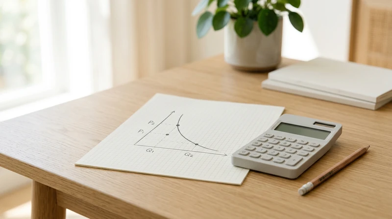
Here is the procedure. Suppose a movie theater raises ticket prices and observes the result:
- Point A: price $10, quantity 1,000 tickets
- Point B: price $12, quantity 800 tickets
Step 1 — percentage change in quantity (midpoint). The change is 800 − 1,000 = −200. The midpoint quantity is (1,000 + 800) ÷ 2 = 900. So the percentage change is −200 ÷ 900 = −0.222, or −22.2%.
Step 2 — percentage change in price (midpoint). The change is $12 − $10 = $2. The midpoint price is (10 + 12) ÷ 2 = 11. So the percentage change is 2 ÷ 11 = 0.182, or +18.2%.
Step 3 — divide. Elasticity = −22.2% ÷ 18.2% = −1.22. Taking the absolute value, the price elasticity of demand is 1.22.
The payoff of the midpoint method: if you ran this in reverse — a price cut from $12 to $10 — you'd get the exact same 1.22, because the denominators are averages, not endpoints.
Reading the Result: Elastic, Inelastic, Unit Elastic
The number itself is only useful if you can interpret it. Compare the absolute value to 1:
- Elastic (elasticity > 1): quantity responds more than proportionally. Our theater result, 1.22, is elastic — an 18.2% price hike cut quantity by 22.2%.
- Inelastic (elasticity < 1): quantity responds less than proportionally. A result of 0.4 means a 10% price rise cuts quantity only 4%.
- Unit elastic (elasticity = 1): quantity changes in exact proportion to price.
Two extremes anchor the scale. Perfectly inelastic demand has an elasticity of 0 — quantity doesn't move at all (a vertical demand curve), as with a life-saving medication. Perfectly elastic demand has an elasticity of infinity — a horizontal curve, where any price rise drops quantity demanded to zero.
Why Elasticity Decides What Happens to Revenue
Elasticity isn't an abstract number — it predicts what a price change does to total revenue (price × quantity). This is the result instructors test most.
When demand is elastic, quantity moves more than price, so a price increase lowers total revenue. The theater example shows it: revenue at Point A was $10 × 1,000 = $10,000; at Point B it was $12 × 800 = $9,600. Raising the price cost the theater $400, exactly because demand was elastic.
When demand is inelastic, quantity barely moves, so a price increase raises total revenue. This is why a subway system can raise fares to bring in more money — riders have few substitutes, demand is inelastic, and revenue climbs. When demand is unit elastic, total revenue stays flat. The rule worth memorizing: with elastic demand, price and revenue move in opposite directions; with inelastic demand, they move together.
What Makes Demand More or Less Elastic
A few factors determine where a good lands on the scale:
- Availability of substitutes. More substitutes mean more elastic demand — a single brand of soda is elastic, but "all soda" is far less so.
- Necessity vs. luxury. Necessities (insulin, electricity) tend to be inelastic; luxuries (concert tickets, restaurant meals) tend to be elastic.
- Share of budget. Goods that eat a large share of income, like rent, have more elastic demand because buyers feel the price more.
- Time horizon. Demand is more elastic in the long run, when buyers have time to find alternatives — gasoline demand barely moves the week prices jump but responds far more over a few years.
Conclusion
To compute price elasticity of demand, divide the percentage change in quantity by the percentage change in price, using the midpoint method so the answer doesn't depend on direction. Then read it against 1: above 1 is elastic, below 1 is inelastic. The single most useful application is revenue — elastic demand means a price hike shrinks revenue, inelastic demand means it grows. For more on what's moving behind the curve, see why the demand curve slopes down.